3.3.2 Costs

Definitions for costs

We can consider costs either in the short run or the long run.

In the short run, at least one factor of production is assumed fixed.

In other words, the quantity of that factor of production remains constant. This means that in the short run, we must distinguish between fixed and variable costs.

In the long run, all factors of production can be varied.

Total costs in the short run

Total cost (TC)= total fixed cost (TFC)+ total variable cost (TVC)

• Total fixed cost refers to costs that do not change with output.
  • So TFC is a horizontal line in the diagram below.
  • Fixed cost examples are costs of renting buildings or costs of capital equipment.
• Total variable cost refers to costs that do change with output.
  • Variable cost examples include workers’ wages and costs of raw materials.
  • For high levels of output, there is an assumption of diminishing marginal product (see below).
  • For low levels of output, there is an assumption of increasing marginal product (see below).

These curves can be drawn as follows:

Average cost in the short run

Average (total) cost = total cost ÷ output. It is the cost per unit produced.

• Similarly, average fixed cost (AFC) = total fixed cost ÷ output.
  • As output increases, the numerator (TFC) is constant but the denominator (output) rises. So overall, the same fixed cost is spread over a larger output base, reducing AFC.
  • In the diagram below, as output rises, AFC falls.
• Average variable cost (AVC) = total variable cost ÷ output.
  • At high output levels, there is diminishing marginal productivity (DMP).
    • DMP- as we increase the amount of the variable factor of production (such as labour), this generates additional output at a decreasing rate.
    • DMP means total cost (and average variable cost) rise at an increasing rate.
    • In other words, as output rises, it becomes more difficult for the firm to increase output. The firm has to use even more inputs to generate the same increase in output.
  • Exam note: It is important to emphasise DMP when explaining why AVC is U shaped.
  • At low output levels, there is increasing marginal product, the opposite of diminishing marginal product. So average variable cost will decrease as output rises.
• Average total cost (AC or ATC) is U shaped:
  • This is because of increasing and diminishing marginal product from the AVC curve.
  • It is also because AFC falls as output rises.
  • Note as output increases, variable costs take up a greater proportion of total costs, as the influence of fixed costs fades. So AVC approaches ATC as output increases.

Marginal cost (MC) is the cost of producing one extra unit of a good.

• MC has the shape of a tick, at first decreasing slightly, then increasing at a higher rate.
• Specifically MC passes through the minimum point of the ATC curve.
  • Consider when MC < ATC. This means the cost of producing the next unit is below the average cost. So producing an extra unit will drag down the average cost. So ATC falls.
  • Consider when MC > ATC. This means the cost of producing the next unit is above the average cost. So producing an extra unit will pull up the average cost. So ATC rises.
  • When MC = ATC, adding an extra unit to production does not move the average. So when MC = ATC, the ATC is minimised.

Link between short-run and long-run cost curves

Difference 1 – fixed versus variable

In the short run at least one factor of production is fixed.

In the long run, all factors of production are variable.

This means there is more flexibility for the firm in its choices of inputs in the long run, compared to the short run. The firm has more choices for how it can change its inputs. So long-run costs are equal or lower than short-run costs in general.

Difference 2 – explanations of U shaped AC curves

Short-run average cost is U shaped, because of diminishing marginal productivity (as well as increasing marginal productivity and falling AFC as output rises).

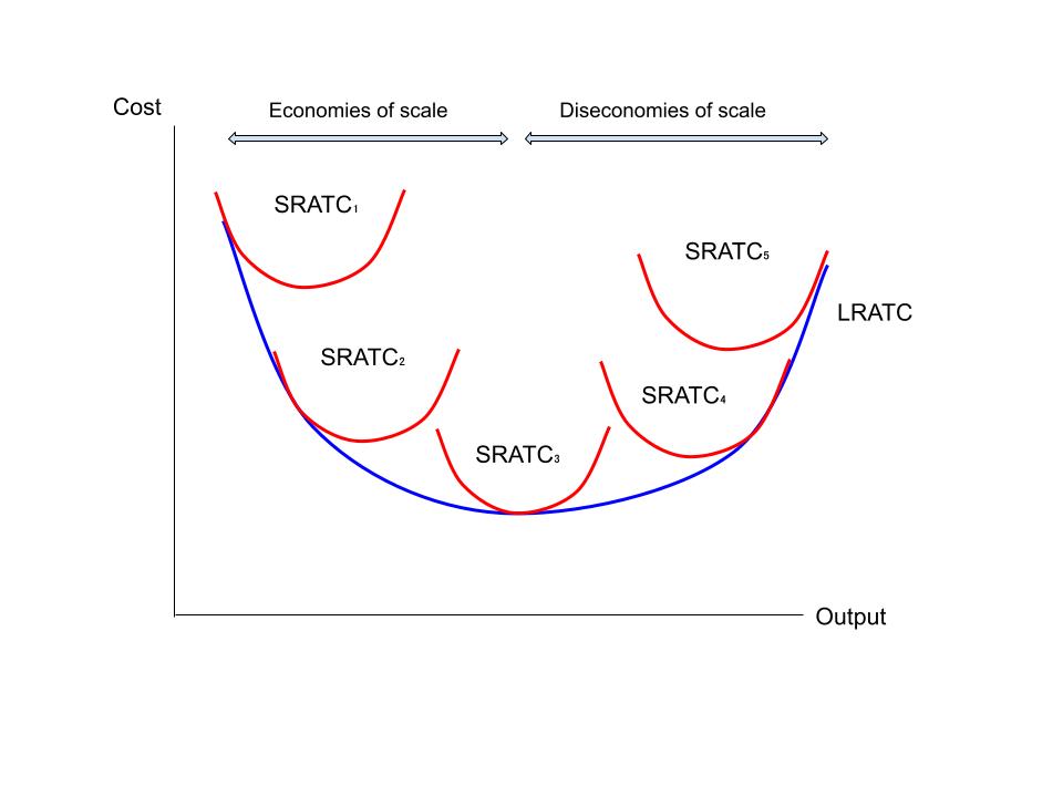
Long-run average cost curves are also U shaped, because of economies and diseconomies of scale.

SRAC and LRAC diagram

There are several SRAC curves. On a given SRAC curve, the level of the fixed factor of production remains the same. However for each unique SRAC curve, there is a different quantity of that fixed factor.

Each short run cost curve has one point that touches the long run average cost curve.

To return to Edexcel Economics A A Level notes, click this button below:

For more A-Level Economics Edexcel A style resources, click the blue button below: